Analytic Methods

Genetics is one of the most quantitative areas of MCAT biology, which is what makes it high-yield: master a handful of analytical tools and you can solve a huge range of passage problems systematically. This guide covers the four core frameworks — Hardy-Weinberg equilibrium, testcrosses, gene mapping by recombination frequency, and basic biometry.

Priority labels: Must know = cold; Know the logic = mechanism not names; Passage-level = recognize, don't memorize; Optional = skippable.

---

Hardy-Weinberg Principle

The Core Idea

Must know

In an idealized population — no mutation, no selection, random mating, infinite size, no migration — allele frequencies stay constant generation to generation. This is Hardy-Weinberg equilibrium (HWE). Its value on the MCAT is as a baseline: a deviation from HWE signals that one assumption is violated (i.e., evolution is occurring), and the MCAT loves asking you to identify which one.

The Five Assumptions

Must know

A population is in HWE only when all hold: no mutation, no natural selection (equal fitness), random mating, no genetic drift (effectively infinite size), no gene flow (no migration). Memory hook: "No M-RADS."

The Equations

Must know

For two alleles with dominant frequency $p$ and recessive frequency $q$:

$p + q = 1$

At equilibrium, genotype frequencies follow:

$p^2 + 2pq + q^2 = 1$

where $p^2$ = homozygous dominant (AA), $2pq$ = heterozygote (Aa), $q^2$ = homozygous recessive (aa). The MCAT almost always gives you $q^2$ (the recessive phenotype is identifiable) and asks you to work backward to $q$, $p$, $2pq$, or $p^2$.

Worked Example

Must know

In a population of 10,000, 400 have cystic fibrosis (autosomal recessive). What fraction are unaffected carriers?

• $q^2 = 400/10{,}000 = 0.04$, so $q = 0.2$
• $p = 1 - q = 0.8$
• Carrier frequency $= 2pq = 2(0.8)(0.2) = 0.32$

So 32% are carriers — far more than the 4% affected. Classic MCAT insight: for rare recessive diseases, carriers vastly outnumber affected individuals.

What HWE Tests on the MCAT

Must know

You may be asked to calculate allele/genotype frequencies from disease prevalence; identify which assumption is violated (small isolated island = drift; assortative mating = non-random mating); or recognize that HWE means frequencies are stable, not equal.

Quick check: A recessive allele has frequency $q = 0.1$ in a population at HWE. What fraction of individuals carry at least one copy?

Answer: Easiest as $1 - p^2 = 1 - 0.81 = 0.19$, or 19%. (Equivalently $2pq + q^2 = 0.18 + 0.01$.) ✓

---

Testcross and the Logic of Mendelian Crosses

Why Testcrosses Matter

Must know

The testcross infers a hidden genotype: cross the unknown against a homozygous recessive ($aa$). Every gamete from the recessive parent carries $a$, so offspring phenotype ratios directly reveal the unknown parent's gamete frequencies — and therefore its genotype.

A backcross is crossing an offspring back to a parent (or parental genotype). A testcross is the special case where that partner is homozygous recessive — so every testcross is a backcross, but not vice versa.

Parental, F1, and F2 Generations

Must know

P = original (often true-breeding) parents; F1 = their offspring (often all heterozygous); F2 = F1 × F1, where Mendelian ratios reappear. A monohybrid cross (Aa × Aa) gives F2 3:1 phenotype, 1:2:1 genotype. A dihybrid cross (AaBb × AaBb) with independent assortment gives F2 9:3:3:1 (9 A_B_ : 3 A_bb : 3 aaB_ : 1 aabb).

Punnett Squares and the Probability Rules

Must know

A Punnett square lays gametes along each axis and fills in offspring genotypes — fine for a monohybrid cross but slow (16 boxes) for dihybrids. For multi-gene problems, use the probability rules instead:

• Product (AND) rule: independent events both occur → multiply. Treat each gene as its own monohybrid cross; e.g., $P(aabb) = \tfrac{1}{4}\times\tfrac{1}{4} = \tfrac{1}{16}$.
• Sum (OR) rule: mutually exclusive events → add. E.g., $P(AA \text{ or } aa) = \tfrac{1}{4}+\tfrac{1}{4} = \tfrac{1}{2}$.

The product rule is far faster for "what fraction of children" questions — e.g., three affected ($aa$) children from $Aa \times Aa$ is $(\tfrac{1}{4})^3 = \tfrac{1}{64}$.

How to Perform a Testcross

Must know

Cross the unknown with a homozygous recessive:

• Unknown AA → all offspring dominant (1 : 0)
• Unknown Aa → 1 dominant : 1 recessive

A dihybrid testcross (AaBb × aabb) with independent assortment predicts 1:1:1:1. Deviation from this is the first signal the genes are linked (see gene mapping).

Epistasis and Modified Ratios

Know the logic

When one gene masks another, the 9:3:3:1 ratio breaks down. You don't need to memorize each variant — just recognize that any F2 ratio deviating from 9:3:3:1 suggests gene interaction.

Optional

Reference: recessive epistasis 9:3:4 (Lab coat color); dominant epistasis 12:3:1; duplicate recessive 9:7; incomplete/codominance 1:2:1 (ABO, snapdragons).

Quick check: A testcross of a dominant-phenotype organism yields 48 dominant and 52 recessive offspring. Most likely genotype of the tested parent?

Answer: The ~1:1 ratio indicates heterozygous (Aa). (If AA, all offspring would be dominant.)

---

Pedigree Analysis

Reading the Symbols

Must know

A pedigree tracks a trait across generations. Squares = males, circles = females, diamond = unspecified sex. Filled = affected, unfilled = unaffected; a dot/half-fill = carrier. A horizontal line joins mates; a vertical line drops to offspring. Generations use Roman numerals, individuals Arabic.

Determining the Inheritance Pattern

Must know

The fast screen: trait skips generations → suspect recessive; appears in every generation → suspect dominant. Then use sex ratio and father-to-son transmission to settle autosomal vs. X-linked.

Pattern	Tell-tale signs
Autosomal recessive	Skips generations; two unaffected parents → affected child; both sexes equally
Autosomal dominant	Every generation; affected child has an affected parent; both sexes equally
X-linked recessive	Mostly males; no father-to-son transmission; affected males trace to carrier mothers
X-linked dominant	Affected father → all daughters, no sons; females ~2× as often
Mitochondrial	Affected mother → all children; affected father → none

(Hemizygosity/sex-linkage mechanics are developed in the Variability guide.)

Quick check: A trait appears every generation, affects both sexes about equally, and an affected father has affected sons. Which pattern?

Answer: Autosomal dominant. Every-generation appearance rules out recessive; father-to-son rules out X-linked; equal sex ratio rules out X-linked dominant and mitochondrial.

---

Gene Mapping: Crossover Frequencies

The Concept: Recombination as a Molecular Ruler

Must know

Genes on the same chromosome are linked (inherited together). During meiosis I, crossing over physically exchanges chromatid segments. The farther apart two genes are, the more likely a crossover separates them — so recombination frequency is a proxy for relative chromosomal distance.

Recombination Frequency and Centimorgans

Must know

$\text{Recombination frequency} = \frac{\text{recombinant offspring}}{\text{total offspring}} \times 100\%$

One centimorgan (cM) = one map unit = the distance giving 1% recombination, so $1\%$ recombination $= 1$ cM. Recombination frequency maxes out at 50% — at that point genes assort independently (as if on separate chromosomes), so genes >~50 cM apart appear unlinked in a testcross.

Two-Point Crosses

Must know

In a testcross (dihybrid × homozygous recessive), count parental classes (same allele combos as the parents; most common) vs. recombinant classes (new combos from crossover; less common).

Example: Linked genes A and B; testcross (AB/ab × ab/ab):

Phenotype	Count	Class
AB	430	Parental
ab	420	Parental
Ab	75	Recombinant
aB	75	Recombinant
Total	1000

$\text{RF} = \frac{75 + 75}{1000} = 15\% \rightarrow 15\text{ cM}$

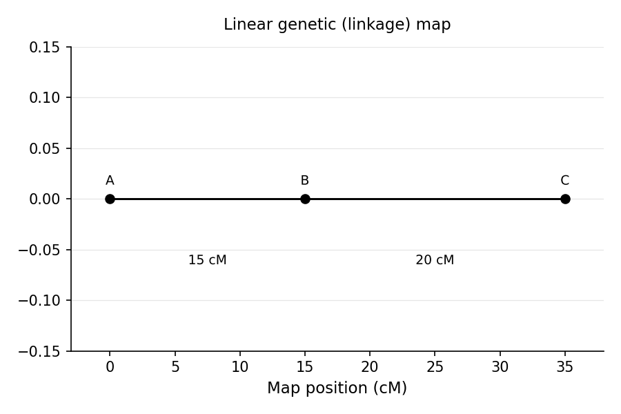
Computing distances between several loci lets you build a linear genetic map with intervals labeled in cM; adjacent short intervals are additive.

Three-Point Crosses and Gene Order

Know the logic

Scoring three genes reveals their order. The double-recombinant classes are always rarest, and the middle gene is the one whose allele is "switched" between a double-recombinant and a parental class. Distance between each adjacent pair is still its recombination frequency. (Double-crossover correction and interference math are beyond the MCAT.)

Quick check: A dihybrid testcross for linked genes yields 200 offspring: 88 + 84 parental, 15 + 13 recombinant. Map distance?

Answer: RF $= (15+13)/200 = 14\%$ → 14 cM.

---

Biometry: Statistical Methods

Why Statistics in Genetics?

Mendelian ratios are probabilistic; real counts vary by chance. Biometry asks: is a deviation from the expected ratio due to chance or to a real biological difference? The MCAT tests this mainly through the chi-square test, plus conceptual mean, variance, and standard deviation.

Two Distinctions to Get Straight First

Must know

Descriptive vs. inferential: descriptive statistics summarize the data you collected (mean, median, SD); inferential statistics (chi-square, t-test) use a sample to draw conclusions about a larger group with a probability attached. Population vs. sample: a population is the whole group of interest; a sample is the subset you measure. You infer population parameters from a sample, which is why a sample mean carries uncertainty (SEM) and larger samples give better estimates.

Descriptive Statistics

Must know

• Mean ($\bar{x}$): arithmetic average; sensitive to outliers.
• Median: middle value; robust to outliers; better for skewed data.
• Mode: most frequent value.
• Variance ($s^2$): average squared deviation from the mean (spread).
• Standard deviation ($s$): $\sqrt{s^2}$. Normal distribution: ~68% within $\pm 1s$, ~95% within $\pm 2s$.
• SEM $= s/\sqrt{n}$: how much the sample mean varies on repetition; shrinks as $n$ grows. Key distinction: SD = spread within data; SEM = precision of the mean estimate.

The t-Test (Comparing Two Means)

Know the logic

Chi-square handles counts in categories; the t-test handles continuous data, asking whether two group means differ more than chance ($H_0$: means equal). If $p < 0.05$, reject $H_0$ (significant). You won't compute it by hand — just recognize that comparing two means (e.g., plant height treated vs. untreated) calls for a t-test, while observed-vs-expected counts call for chi-square.

The Chi-Square ($\chi^2$) Test

Must know

Tests whether observed counts fit a hypothesized Mendelian ratio. $H_0$: the data match the expected ratio (e.g., 3:1).

$\chi^2 = \sum \frac{(O - E)^2}{E}$

Degrees of freedom = number of classes $- 1$. Compare your $\chi^2$ to a critical value (the MCAT provides the table; usually $p = 0.05$):

• $\chi^2 \leq$ critical value → fail to reject $H_0$ → deviation likely chance → data consistent with the ratio
• $\chi^2 >$ critical value → reject $H_0$ → significant deviation → data do not fit

Worked Chi-Square Example

Must know

A monohybrid F2 yields 740 dominant, 260 recessive (total 1000); test against 3:1. Expected: 750 dominant, 250 recessive.

$\chi^2 = \frac{(740-750)^2}{750} + \frac{(260-250)^2}{250} = 0.133 + 0.400 = 0.533$

df $= 2 - 1 = 1$; critical value ≈ 3.84. Since $0.533 < 3.84$, fail to reject $H_0$ — consistent with 3:1.

Statistical Significance vs. Biological Significance

Know the logic

A result can be statistically significant (p < 0.05) yet biologically trivial (tiny effect detectable only with huge $n$); conversely, a real effect may miss significance in an underpowered (small $n$) study.

Quick check: A dihybrid F2 yields 580 A_B_, 180 A_bb, 170 aaB_, 70 aabb (total 1000); chi-square vs. 9:3:3:1 gives $\chi^2 = 1.8$, df = 3, critical value ≈ 7.81. Conclusion?

Answer: Since $1.8 < 7.81$, fail to reject $H_0$ — consistent with 9:3:3:1; no evidence for linkage or epistasis.

---

Common Confusions & Tricks

1. $q^2$ is your entry point into HWE — but confirm the trait is autosomal recessive.
For X-linked traits the equations apply differently (females $p^2$, $2pq$, $q^2$; males just $p$ and $q$, being hemizygous). Don't apply the standard equation to X-linked males.

2. Recombination frequency ≠ physical distance.
50 cM doesn't mean opposite ends of one chromosome — they could be on different chromosomes. Genes >50 map units apart appear unlinked. Distances are additive only for short intervals; long intervals underestimate true distance (double crossovers cancel out).

3. "Fail to reject" ≠ "accept" the null.
You never prove the null. "The data are consistent with a 3:1 ratio" is correct; "the data prove a 3:1 ratio" is not.

4. Standard deviation vs. standard error.
SD = variability in raw data; SEM = SD/√n = precision of the mean. "±SEM" error bars shrink as n grows; "±SD" bars do not.

5. Parental vs. recombinant classes.
Parental classes are most common. Asked which are recombinant? Pick the two least-frequent classes.

6. The 1:1:1:1 vs. 1:1 testcross ratio.
Unlinked dihybrid testcross → 1:1:1:1. Completely linked (no crossing over) → only two parental classes 1:1. Partial linkage → four classes, unequal.

7. Chi-square uses counts, never proportions.
Convert percentages back to raw numbers before calculating.

8. HWE trick: $p^2 + q^2 = 1 - 2pq$.
Homozygote frequency = one minus heterozygote frequency. Useful for "proportion NOT carriers."

---

Key Takeaways

Hardy-Weinberg Equilibrium

• Core equations: $p + q = 1$ and $p^2 + 2pq + q^2 = 1$
• Five assumptions (No M-RADS): no mutation, random mating, no drift, no selection, no gene flow
• Workflow: $q^2$ = affected frequency → $q$ → $p = 1 - q$ → $2pq$ = carrier frequency
• Carriers ($2pq$) far exceed affected ($q^2$) for rare recessive alleles

Testcross and Generational Notation

• P → F1 → F2; F1 typically heterozygous; F2 = 3:1 (monohybrid) or 9:3:3:1 (dihybrid)
• Testcross = unknown × homozygous recessive; offspring ratio reveals parental gamete frequencies
• Modified 9:3:3:1 ratios (9:3:4, 12:3:1, 9:7) signal epistasis

Gene Mapping

• Recombination frequency (%) = map distance in cM
• RF = (recombinant offspring / total) × 100%; maxes at 50% (independent assortment above this)
• Double recombinants are rarest; the middle gene is the "switched" allele in double recombinants

Biometry

• Descriptive summarizes a sample; inferential (chi-square, t-test) generalizes sample → population with a probability
• Mean (sensitive to outliers), median (robust), mode, SD (spread), SEM = SD/√n (precision of mean)
• Normal distribution: ±1 SD ≈ 68%, ±2 SD ≈ 95%
• Chi-square: $\chi^2 = \sum (O-E)^2/E$; df = classes − 1; $H_0$ = data fit the expected ratio
• $\chi^2 \leq$ critical → fail to reject (consistent); $\chi^2 >$ critical → reject (significant deviation)
• Statistical significance ≠ biological significance